VNA Automatic Calibration via SCPI

Introduction

This chapter describes how to automate the calibration process of a Vector Network Analyzer (VNA) using Standard Commands for Programmable Instruments (SCPI) and Python.

Calibration is the most critical step in RF measurements. It mathematically removes the systematic errors (Directivity, Source Match, and Reflection Tracking) introduced by the VNA hardware and cables, shifting the measurement plane to the end of the test port.

Objectives

This tutorial serves two primary purposes:

1. Practical Application: To perform a “Full One-Port” (FOPort) automatic calibration required for accurate reflection measurements (S11) up to 18 GHz.

2. Skill Development: To provide a hands-on example of how to communicate with high-end test equipment using the PyVISA library and raw SCPI strings.

System Requirements

• Hardware: Rohde & Schwarz ZNL series VNA and a compatible Automatic Calibration Unit (e.g., ZN-Z151).

• Connection: Ethernet (TCP/IP) via HiSLIP protocol.

• Libraries: pyvisa, numpy.

Implementation

The following Python script initializes the instrument, sets the frequency sweep from 100 MHz to 18 GHz, and triggers the internal AutoCal routine.

import pyvisa

# Initialize communication
rm = pyvisa.ResourceManager()
vna = rm.open_resource('TCPIP0::10.0.0.5::hislip0::INSTR')
vna.timeout = 120000  # Calibration hardware takes time to switch internal states

# Reset the instrument to default state
vna.write("*RST")

# Set frequency range: 100 MHz to 18 GHz
vna.write("SENSe1:FREQuency:STARt 100e6")
vna.write("SENSe1:FREQuency:STOP 18e9")
vna.write("SENSe1:SWEep:POINts 1601")

# Run autocal on port 1 using factory characterization ('')
# The VNA automatically detects the CalUnit connected to Port 1
vna.write("SENSe1:CORRection:COLLect:AUTO '', 1")

# *OPC? is vital: it pauses the script until the VNA hardware is finished
vna.query("*OPC?")

# Verify calibration status
state = vna.query("SENSe1:CORRection:STATe?").strip()
print(f"Calibration active: {state}")  # 1 = Success/Active

# Save the resulting calibration data to the internal storage
vna.write("MMEMory:STORe:CORRection 1, 'AutoCal_Port1.cal'")

vna.close()
rm.close()

# Later load with
#vna.write("MMEMory:LOAD:CORRection 1, 'AutoCal_Port1.cal'")

Command Breakdown

• SENSe1:CORRection:COLLect:AUTO '', 1: The empty string tells the VNA to use the factory data stored inside the CalUnit. The 1 specifies the physical Port 1 of the VNA.

• *OPC?: Stands for “Operation Complete.” It prevents the script from closing the session before the physical switches inside the CalUnit have finished cycling.

Extracting and Verifying Calibration Error Terms

Once a calibration is performed and saved, it is often necessary to verify the quality of the calibration or extract the error terms for offline analysis. The following script demonstrates how to load a previously saved calibration file and retrieve the Directivity, Source Match, and Reflection Tracking coefficients.

import pyvisa
import numpy as np
import skrf as rf

rm = pyvisa.ResourceManager()
vna = rm.open_resource('TCPIP0::10.0.0.5::hislip0::INSTR')
vna.timeout = 100000

# Reset and load the specific calibration file
vna.write("*RST")
vna.write("MMEMory:LOAD:CORRection 1, 'AutoCal_Port1.cal'")

# Verification Queries
print(f"Is AutoCal: {vna.query('SENSe1:CORRection:DATA:PARameter? ACAL')}")
print(f"Cal Date: {vna.query('SENSe1:CORRection:DATE?')}")

# Set to HOLD mode to ensure data consistency during readout
vna.write("SENSe1:SWEep:MODE HOLD")

# Request raw error term data
D_raw = vna.query("SENSe1:CORRection:CDATa? 'DIRECTIVITY', 1, 0")
S_raw = vna.query("SENSe1:CORRection:CDATa? 'SRCMATCH', 1, 0")
R_raw = vna.query("SENSe1:CORRection:CDATa? 'REFLTRACK', 1, 0")

# Data Transformation: From String to Complex Array
D_complex = np.array(D_raw.split(','), dtype=float)
D_complex = D_complex[0::2] + 1j * D_complex[1::2]

S_complex = np.array(S_raw.split(','), dtype=float)
S_complex = S_complex[0::2] + 1j * S_complex[1::2]

R_complex = np.array(R_raw.split(','), dtype=float)
R_complex = R_complex[0::2] + 1j * R_complex[1::2]

print(f"Points Extracted: {len(D_complex)}")
print(f"First Directivity Point: {D_complex[0]}")

vna.write("SENSe1:SWEep:MODE CONTinuous")

#Converting error terms to Network objects for visualizing them using Sci kit RF

freq = rf.Frequency(start=100e6, stop=18e9, npoints=1601, unit='Hz')
ntwk_D = rf.Network(frequency=freq, s=D_complex, name='Directivity')
ntwk_S = rf.Network(frequency=freq, s=S_complex, name='Source Match')
ntwk_R = rf.Network(frequency=freq, s=R_complex, name='Refl Tracking')


plt.figure(figsize=(15, 5))

plt.subplot(1, 3, 1)
ntwk_D.plot_s_db()
plt.title('Directivity (ED)')

plt.subplot(1, 3, 2)
ntwk_S.plot_s_db()
plt.title('Source Match (ES)')

plt.subplot(1, 3, 3)
ntwk_R.plot_s_smith()
plt.title('Reflection Tracking (ER)\n(Smith Chart)')

plt.tight_layout()
plt.show()


vna.close()
rm.close()

Understanding the Data Transition: D_raw to D_complex

The transition from the raw string returned by the VNA to a usable complex mathematical array in Python happens in three distinct stages:

1. String Splitting and Type Casting

When the VNA executes CDATa?, it returns a single, massive string of comma-separated values (e.g., "0.012,-0.005,0.011,...").

• D_raw.split(','): Breaks the string into a Python list of individual substrings.

• np.array(..., dtype=float): Converts those substrings into 64-bit floating-point numbers.

2. De-interleaving with Slicing

VNA hardware communicates complex data in an interleaved format: [Real_1, Imag_1, Real_2, Imag_2, ...]. To perform vector math, we must separate these.

• D_complex[0::2]: This uses NumPy slicing to start at index 0 and take every 2nd element. This captures all Real components.

• D_complex[1::2]: This starts at index 1 and takes every 2nd element. This captures all Imaginary components.

3. Complex Vector Reconstruction

The final step uses the imaginary unit 1j (the Python equivalent of \(i\)) to rebuild the vectors:

\[D_{complex} = Real + j \cdot Imaginary\]

By adding the two sliced arrays together with the 1j multiplier, NumPy creates a single array of complex128 objects. This allows you to calculate Magnitude (np.abs()) and Phase (np.angle()) directly, which is essential for analyzing systematic errors at high frequencies like 18 GHz.

Visualization of Error Terms

After extracting the complex coefficients, we can visualize the VNA’s internal state. These plots provide insight into the quality of the calibration and the physical characteristics of the test setup.

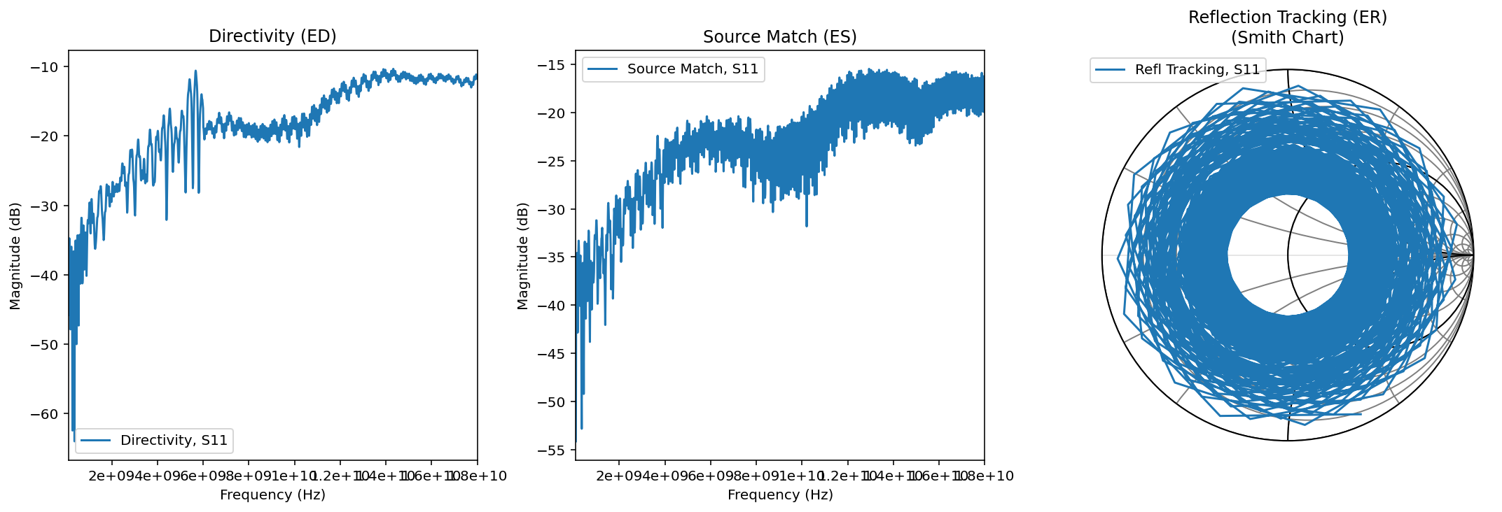
Figure 1: Log-Magnitude plots of Directivity and Source Match, alongside a Smith Chart representation of Reflection Tracking.

Data Interpretation

• Directivity (ED): Represents the leakage within the VNA. A value moving from -50 dB toward -15 dB at 18 GHz is typical, showing reduced isolation at higher frequencies.

• Source Match (ES): Shows the reflections looking back into the VNA port. The values between -35 dB and -18 dB indicate a healthy match for a standard cable assembly.

• Reflection Tracking (ER): The “spiral” seen on the Smith Chart is the result of the phase delay introduced by the cables and PCB traces. At 18 GHz, the signal undergoes multiple full rotations of phase, which the VNA mathematically tracks to shift the measurement plane to your device.